FEA: Transient Structural
This tutorial computes the structural response to a time-dependent pulse. The same geometry, material, support, and load concepts used in Static Structural apply here, but the solver advances through time so you can see the peak response and how it decays.
What you will learn
- Prepare the supplied component for a time-dependent structural solve.
- Set total time, time step, and Rayleigh damping parameters.
- Run the transient solver and track its progress.
- Animate displacement and equivalent stress through the time steps.
- Apply color maps and read peak values and time-history charts.
1. Geometry and material
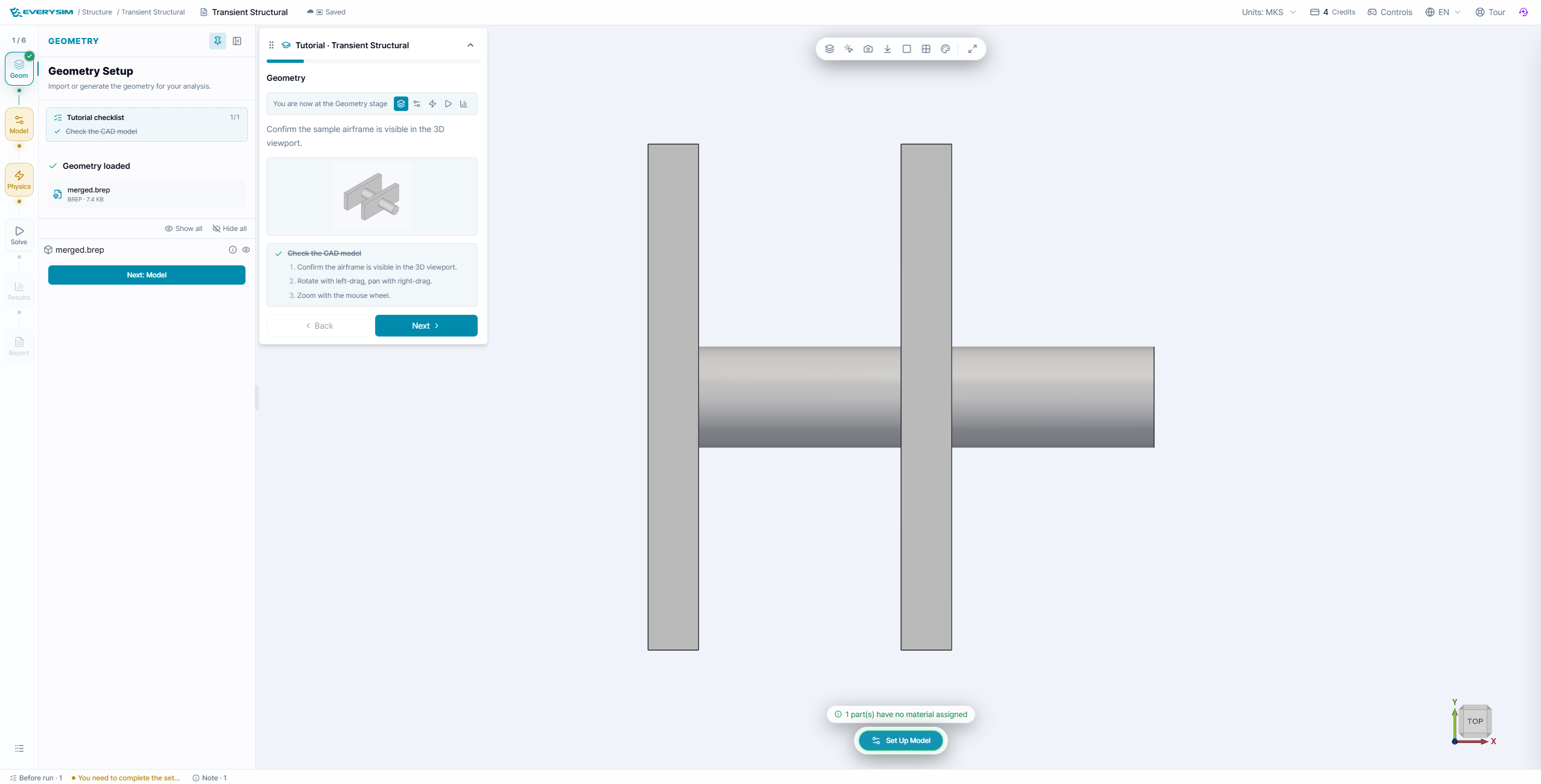
Confirm that the bracket/shaft sample is loaded and that the plates, connector, and shaft are visible. Assign the tutorial material to every body.
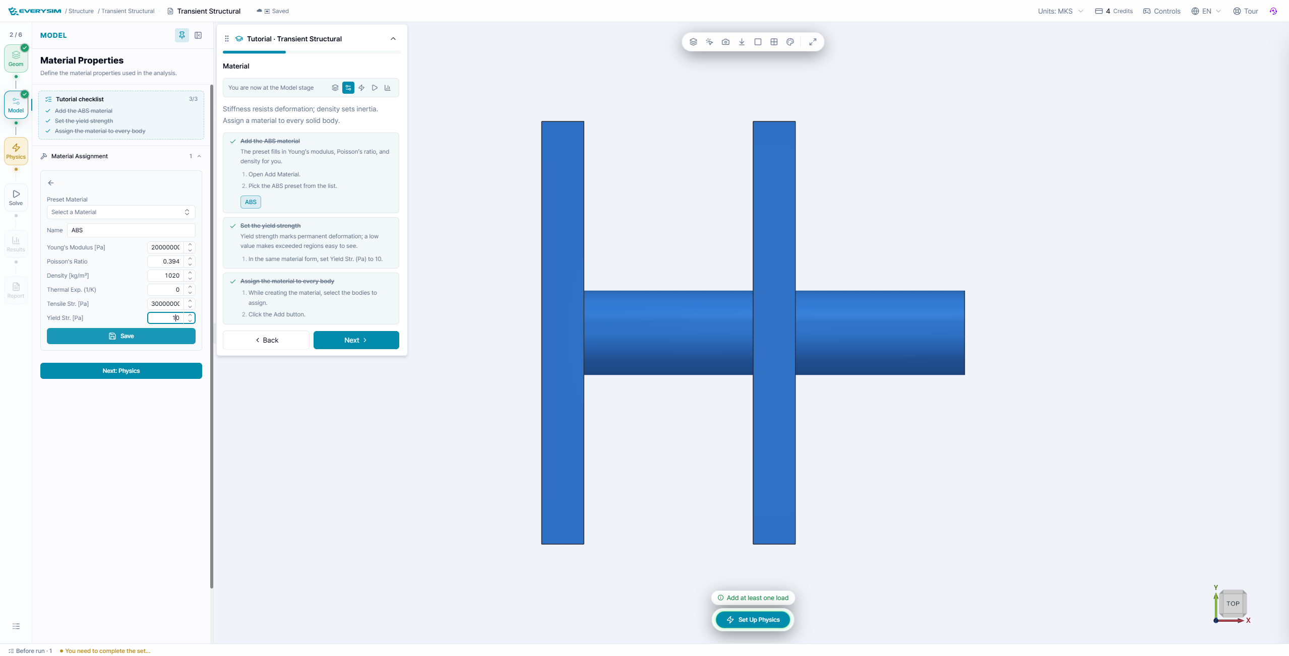
Material density and stiffness both affect the transient response. Check the material card before continuing, especially if you later replace the tutorial material with a flight hardware material.
2. Support and time-varying load
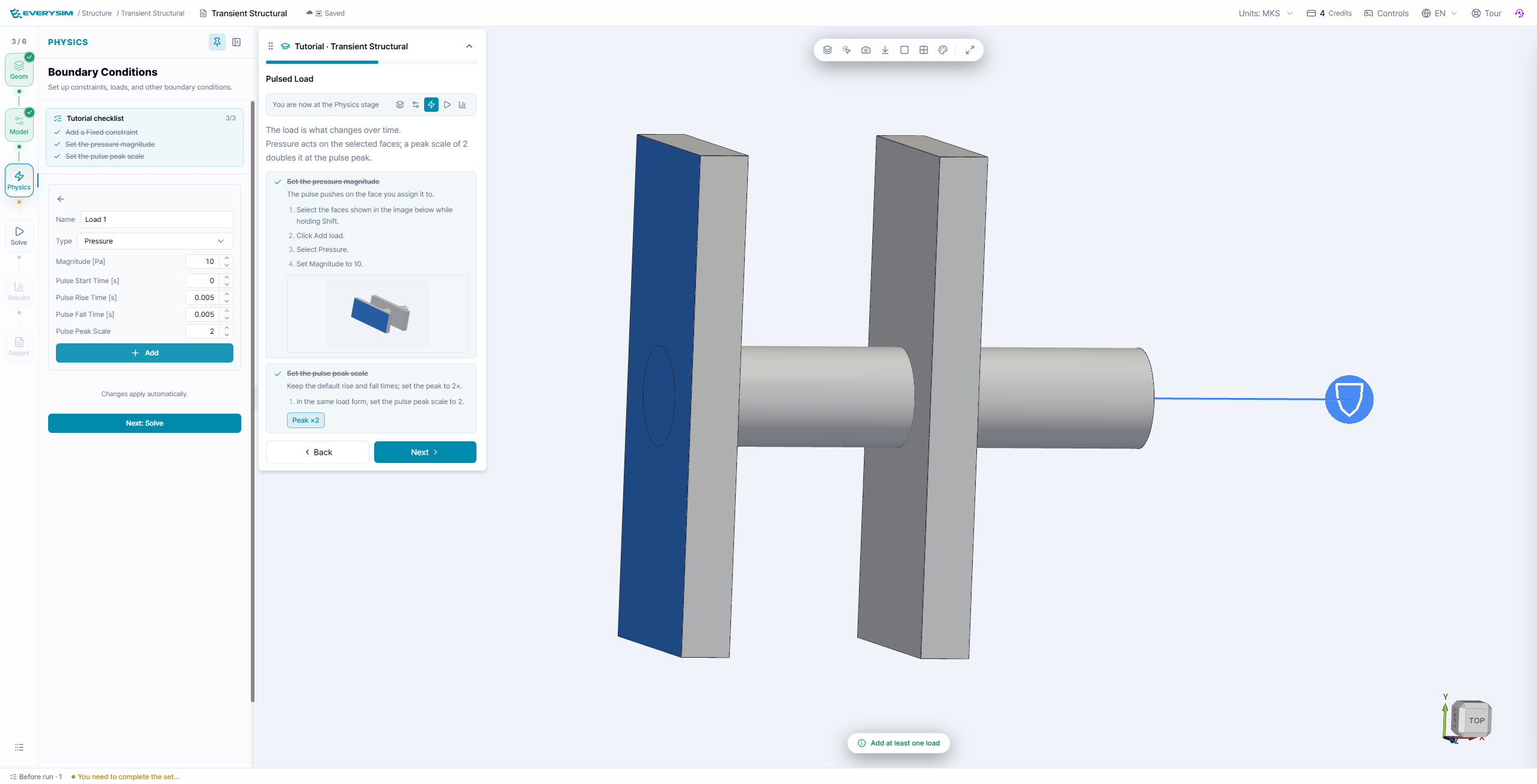
In Physics, apply the tutorial fixed support to the indicated face and define the time-dependent load on the highlighted face. Verify the arrow direction and the load unit before solving.
The load history is applied over the total analysis time. A transient run can show a high short-lived response even when the final response is small, so do not evaluate only the last frame.
3. Transient parameters and solve
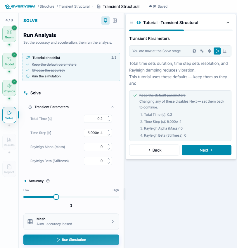
Keep the tutorial values:
- Total Time:
0.2 s. - Time Step:
5.000e-4 s. - Rayleigh Alpha (Mass):
0. - Rayleigh Beta (Stiffness):
0. - Accuracy:
3.
Total time controls how long the event is simulated. Time step controls temporal resolution: a smaller step captures faster changes but increases solve cost. Rayleigh coefficients add proportional damping; zero keeps the tutorial response undamped by those terms.
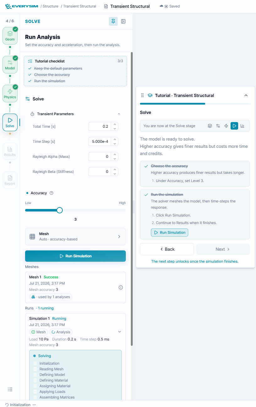
Click Run Simulation and wait for both mesh and analysis to finish. The run card shows the load, duration, time step, and mesh accuracy; use it to confirm that the result corresponds to the intended case.
4. Results: displacement and stress history
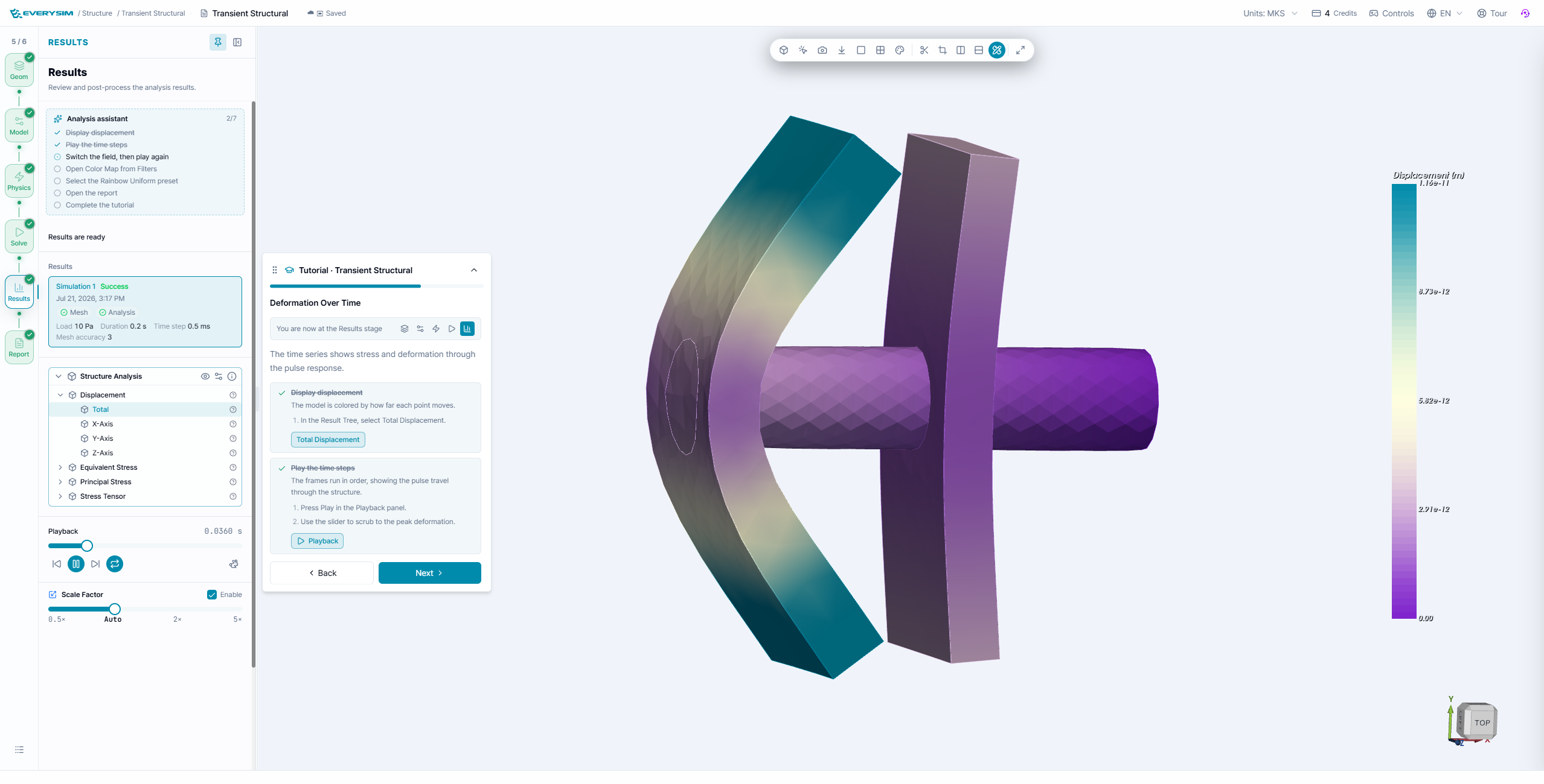
Select Total Displacement and use the playback controls. The slider selects a time step; Play shows how the pulse travels through the structure. Use Scale Factor only to make the shape visible—the scale does not change the numerical result.
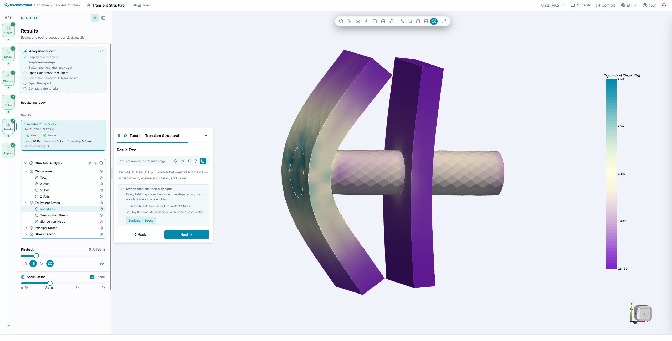
Switch to Equivalent Stress or von Mises and replay the same time steps. Comparing stress and displacement at the same time helps identify whether a peak is caused by rigid motion, bending, or local stress concentration.
5. Color maps
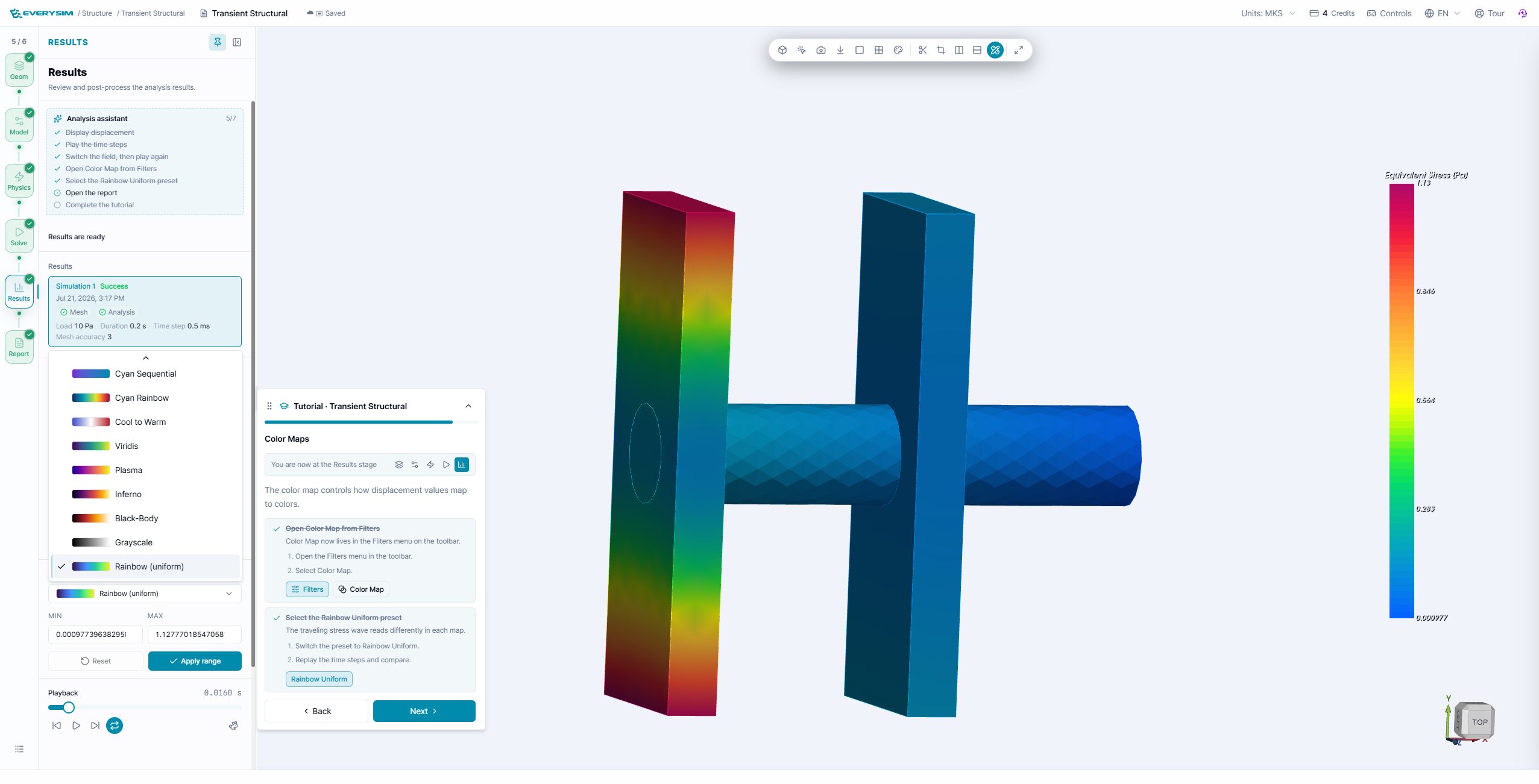
Open Filters → Color Map and choose Rainbow (uniform) or another consistent preset. Use the same range when comparing time steps; automatic rescaling can make two frames look equally severe even when their magnitudes differ.
6. Report and time histories
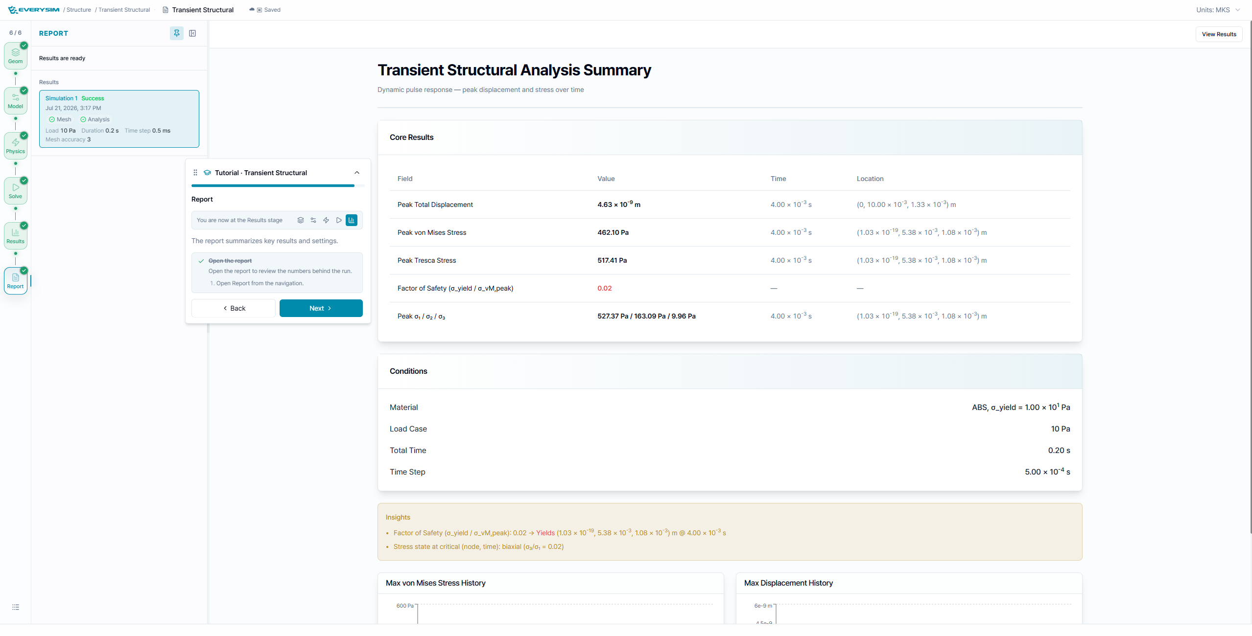
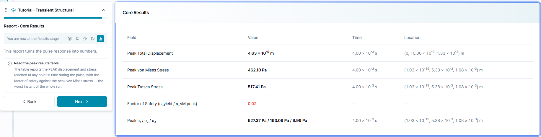
The report records the peak total displacement, peak von Mises stress, peak Tresca stress, factor of safety, critical time, and critical location. In the example screenshot, the peaks occur near 4.00 × 10⁻³ s, not at the end of the 0.2 s run.
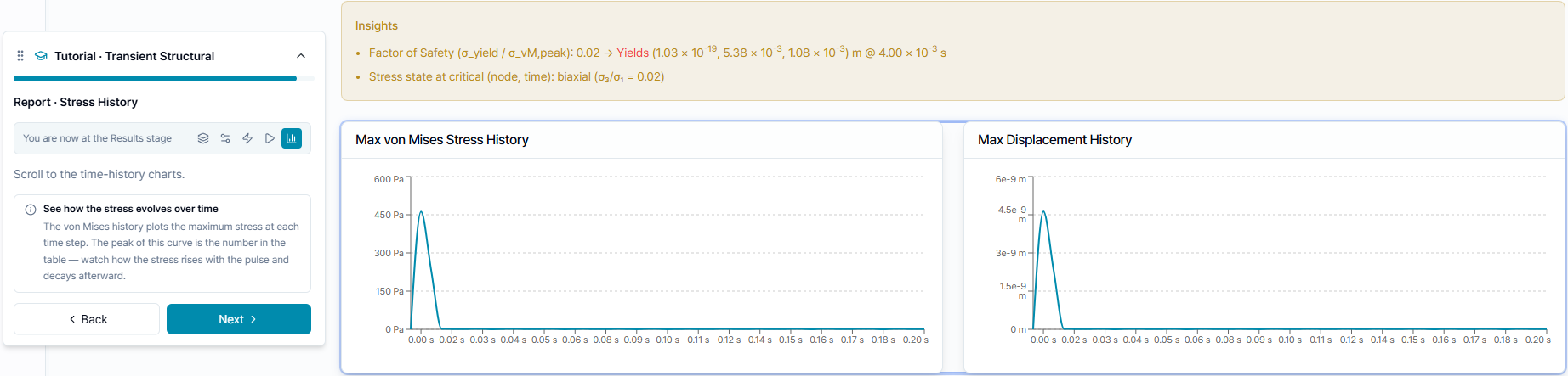
Read the history charts to see the pulse rise and decay. If a peak occurs between saved frames, refine the time step and repeat the run before using the result for design decisions.
Interpretation checklist
- Confirm that the physical load history and units are correct.
- Check the first and peak time steps, not only the final frame.
- Keep total time and time step consistent when comparing designs.
- Treat a low factor of safety as a prompt to review material and loading assumptions, especially at a transient peak.