CFD: External Flow
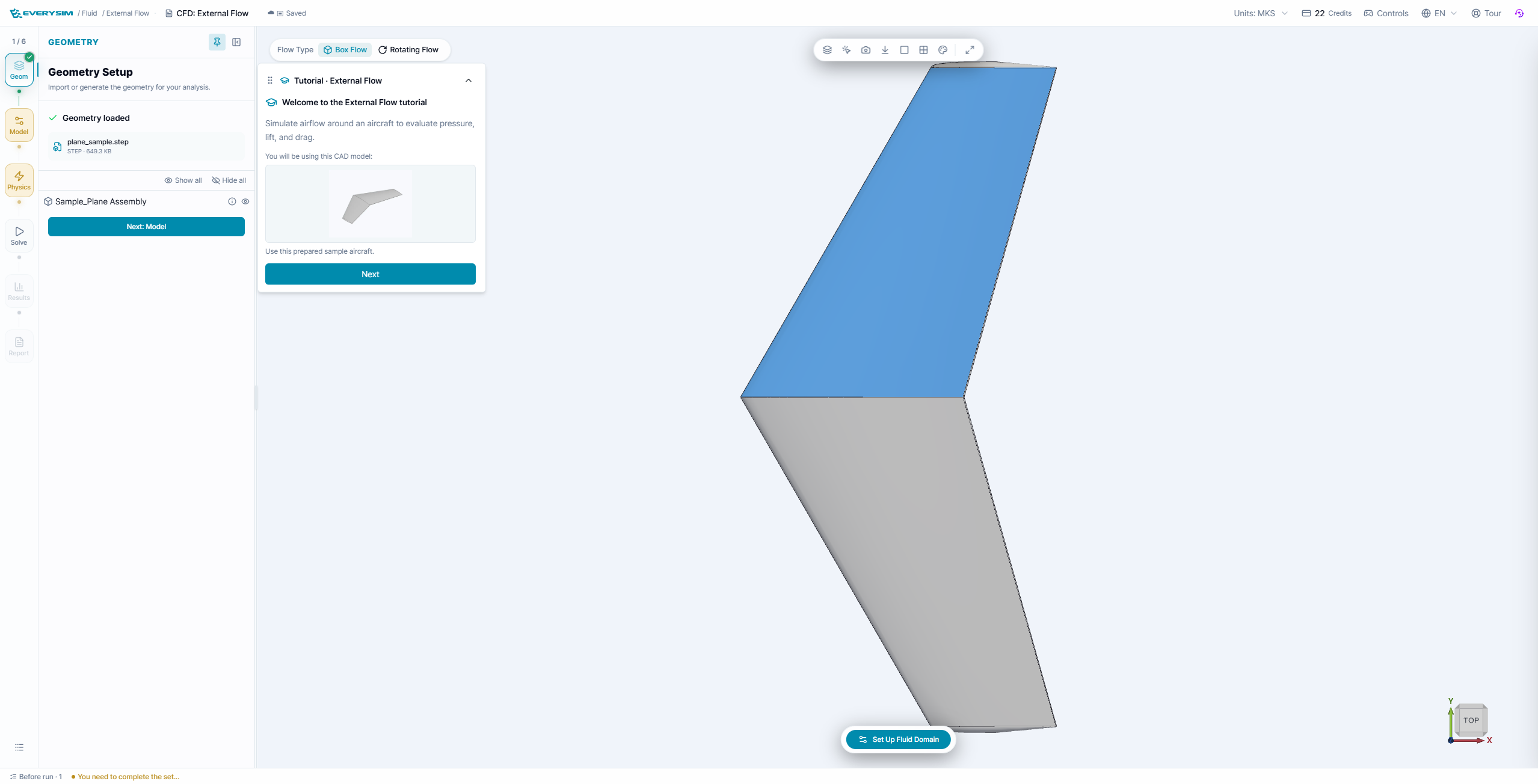
This tutorial shows how to run an external aerodynamics simulation around a fixed-wing aircraft body. You will set a box flow domain, define freestream conditions, run a CFD analysis, inspect result fields, create a cut plane, save the section, enable streamlines, and read the aerodynamic report.
What You Will Learn
- Confirm the prepared fixed-wing CAD model.
- Build a Box Flow domain around the aircraft.
- Set wind speed, angle of attack, sideslip, flow direction, and lift direction.
- Choose accuracy and acceleration settings before solving.
- Monitor residuals while the mesh and analysis run.
- Review pressure, velocity, turbulence, vorticity, wall shear stress, and other CFD fields.
- Use Cut and Streamline tools to inspect the internal flow structure.
- Read lift, drag, force, and moment report sections.
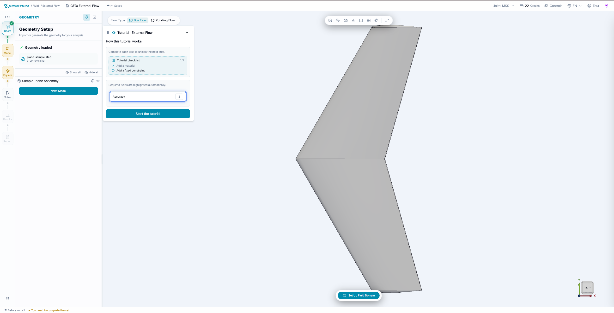
The in-workbench tutorial panel highlights the required fields and keeps the checklist synchronized with the current stage.
1. Geometry
The tutorial starts with plane_sample.step already imported. The model appears in the Geometry stage as Sample_Plane Assembly.
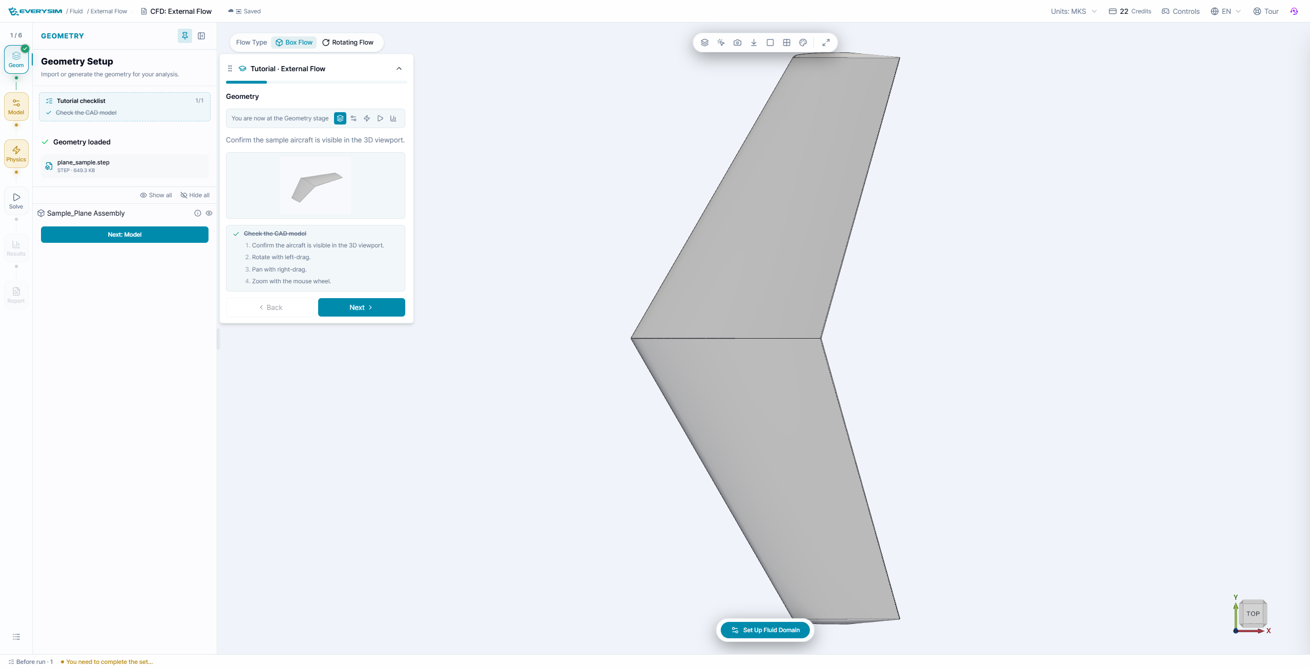
- Open the Geometry stage.
- Confirm that Geometry loaded is checked.
- Verify that
plane_sample.stepappears in the file list. - Rotate, pan, and zoom the 3D viewport to confirm that the model is visible.
This stage is only a readiness check; the tutorial uses the prepared sample aircraft.
2. Model: Flow Domain
In the Model stage, define the air volume around the aircraft. For this tutorial, use Box Flow because the aircraft is moving through still air.
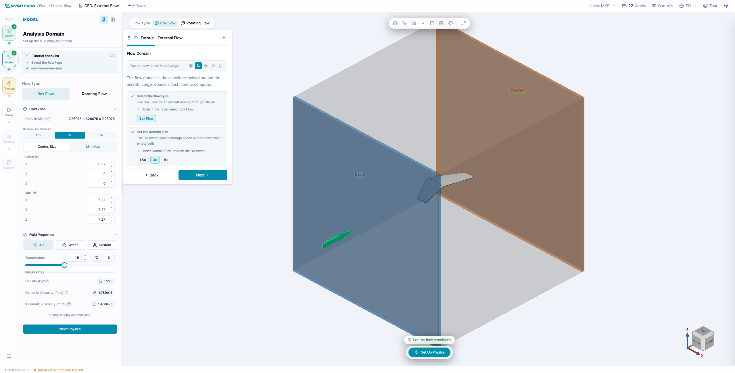
- In Flow Type, select Box Flow.
- Under Domain Size, choose the 3x preset.
- Keep the domain centered around the aircraft unless your tutorial checklist asks for a different value.
- Use Air as the fluid property.
- Keep the default air properties unless you need to model a different environment.
The domain preview shows the inlet and outlet faces. The inlet side is where the air enters the domain, and the outlet side is where it exits after passing around the aircraft.
3. Physics: Flow Conditions
Use the Physics stage to define the incoming flow and aircraft orientation.
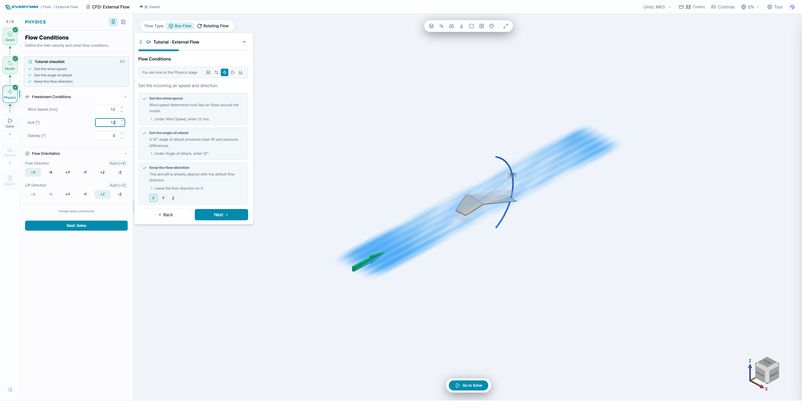
Recommended tutorial settings:
- Wind Speed: 12 m/s
- Angle of Attack: 12 degrees
- Sideslip: 0 degrees
- Flow Direction: Auto (+X)
- Lift Direction: Auto (+Z)
The 3D preview displays blue flow streaks and an angle-of-attack guide around the aircraft. This lets you confirm that the incoming air direction and lift direction are aligned before solving.
4. Solve
The Solve stage controls result quality, CPU usage, and run submission.
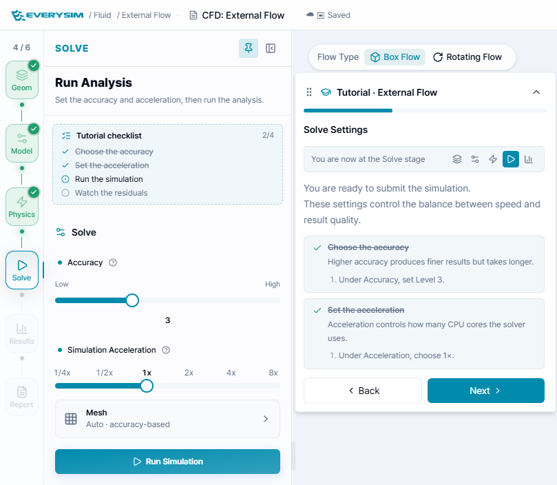
- Set Accuracy to 3.
- Set Simulation Acceleration to 1x.
- Confirm that the mesh is set to Auto - accuracy-based.
- Click Run Simulation.
After the run begins, the workbench creates the mesh and starts the analysis. The left panel shows mesh progress, analysis status, and run cards.
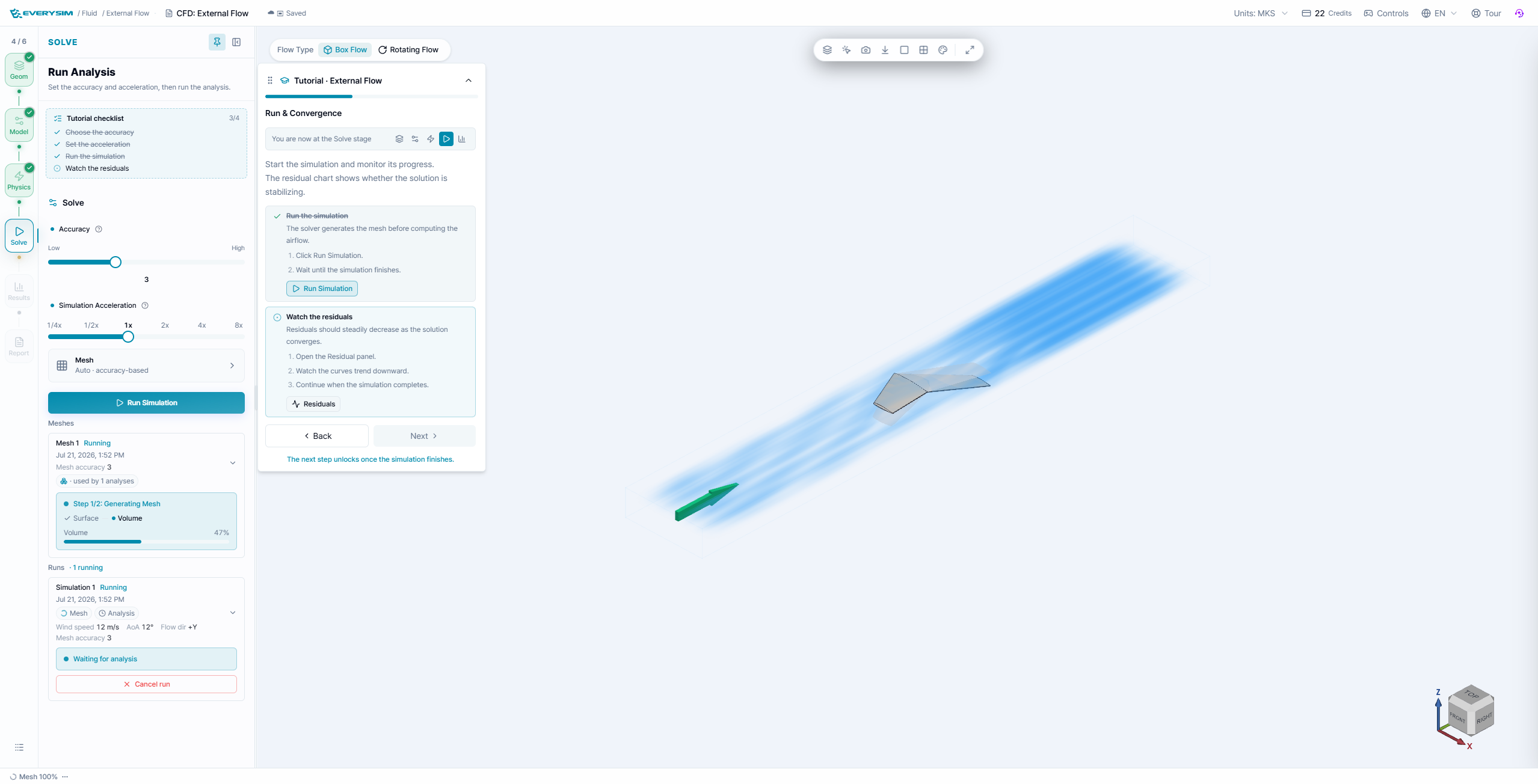
Open Residuals while the analysis runs. Residual curves show whether the solution is stabilizing.
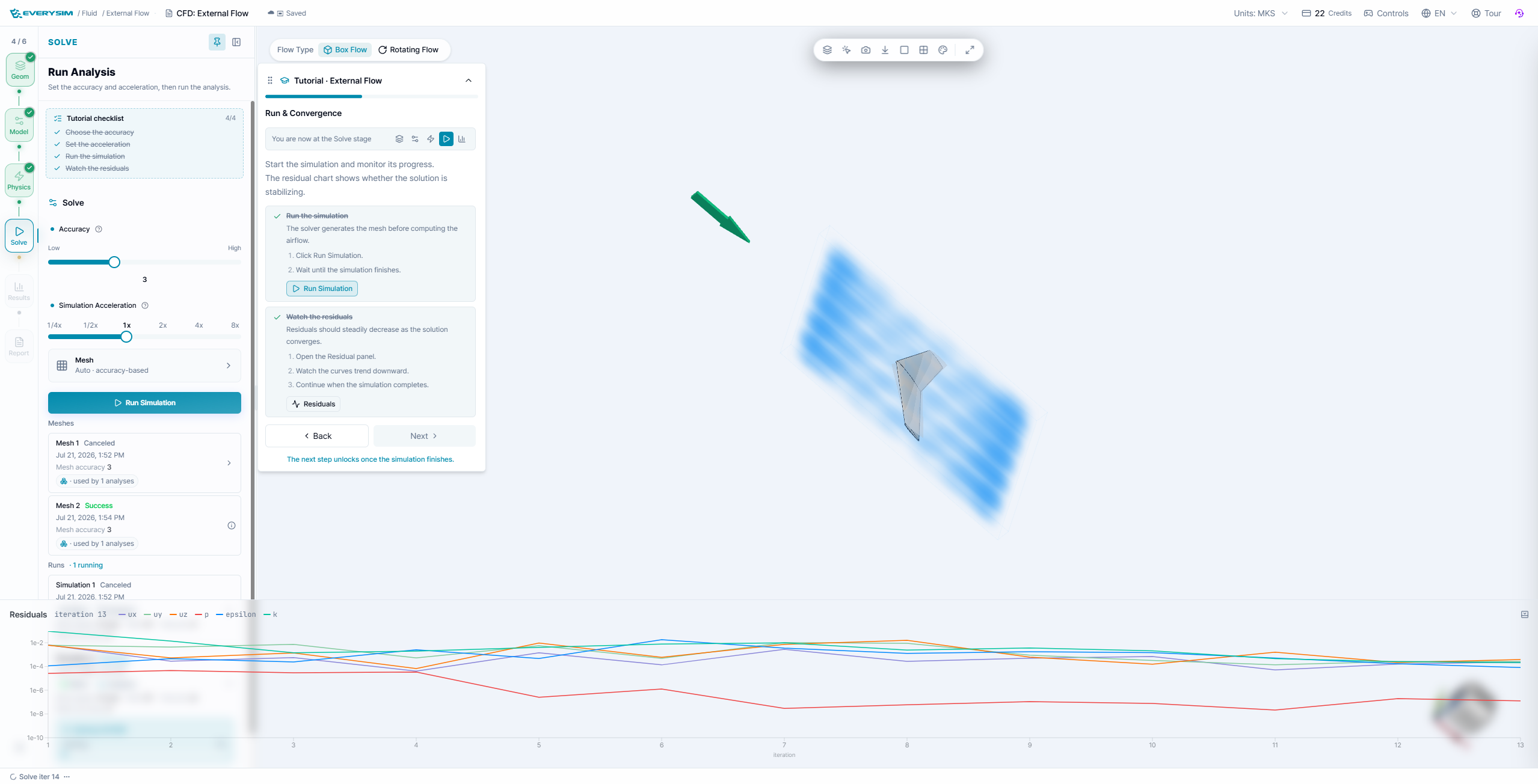
Use residuals as a convergence indicator, but do not judge the run only from the chart. Also inspect the final flow fields and force trends in the report.
5. Results: Field Review
When results are ready, the Results stage lists the computed fields. Typical fields include Velocity, Pressure, Turbulence (k), Turbulence (μt), Turbulence (ε), Q-criterion, Vorticity, and Wall Shear Stress.
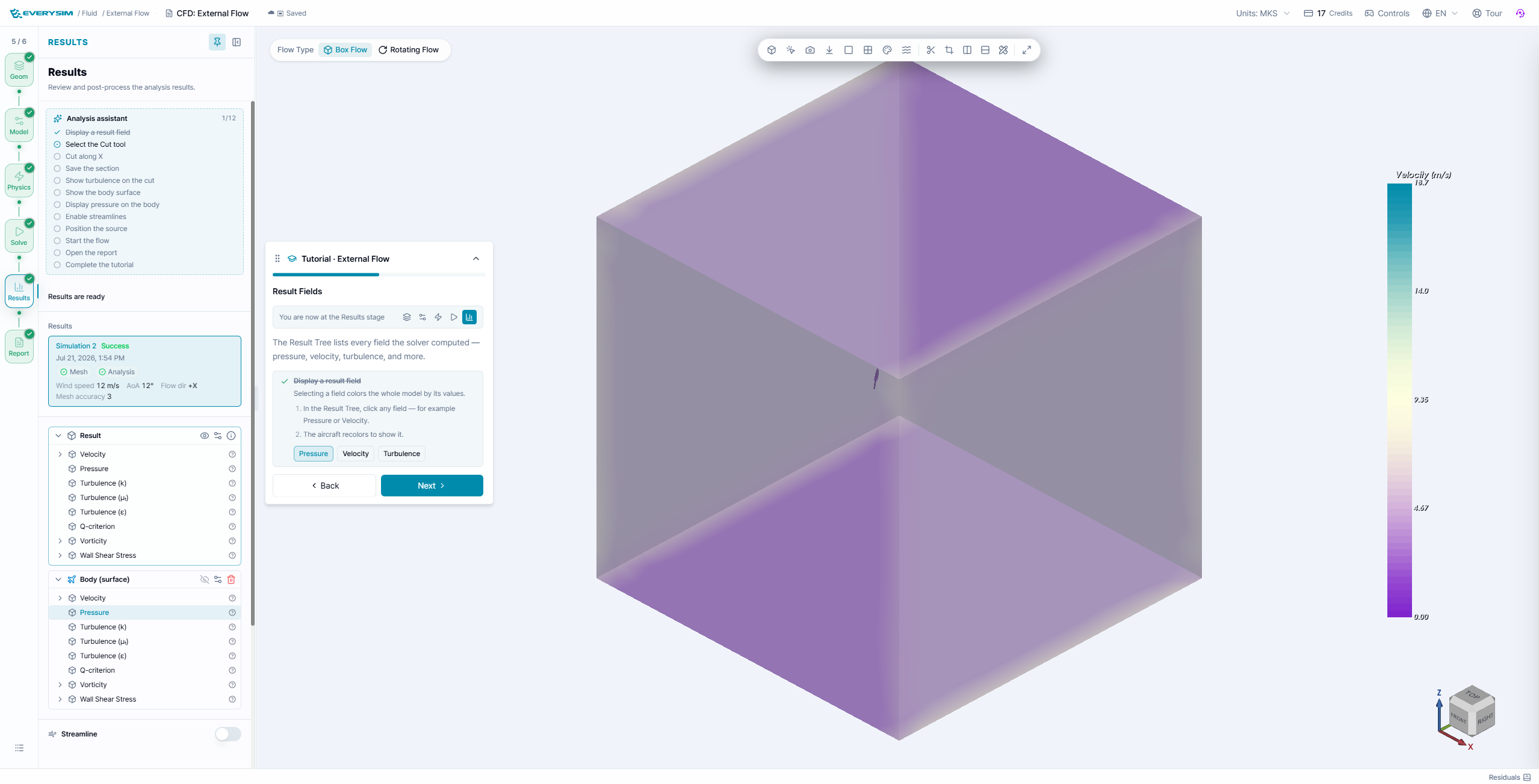
Start with a broad field:
- In the Result Tree, select Pressure or Velocity.
- Confirm that the model is colored by the selected field.
- Use the color legend to compare high and low regions.
- Toggle result entries on or off to isolate the aircraft body, domain, cut plane, or saved sections.
Pressure is useful for lift and drag interpretation. Velocity is useful for identifying acceleration around the body and flow changes near the wake.
6. Results: Cut Plane and Saved Section
A cut plane reveals internal values in the flow volume, not just values on the aircraft surface.
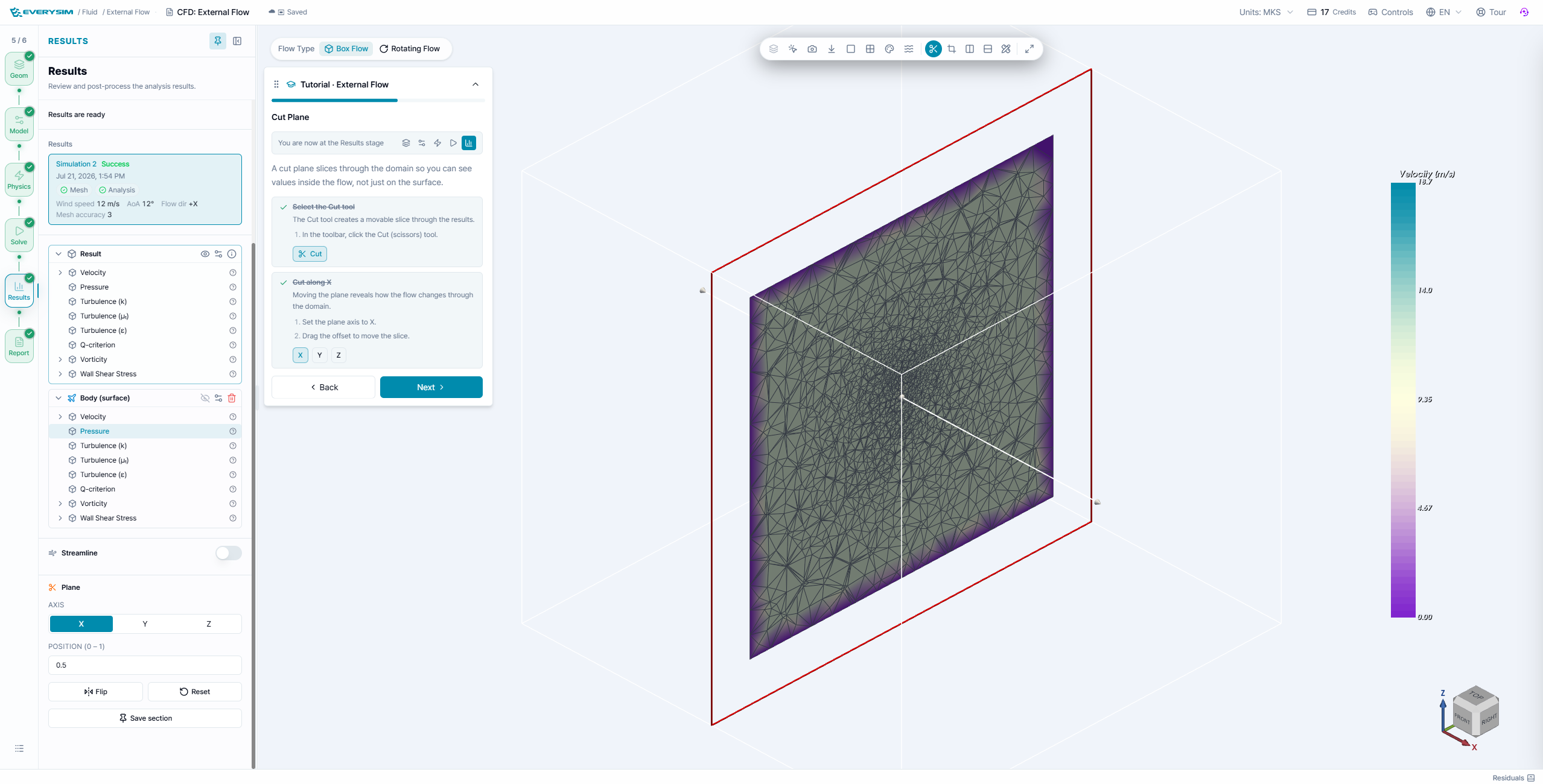
- Select the Cut tool from the toolbar.
- Choose the cut axis. The tutorial uses X.
- Move the plane position to reveal the area you want to inspect.
- Use Flip or Reset if the section orientation needs adjustment.
Save the cut as its own result entry when you want to analyze it independently.
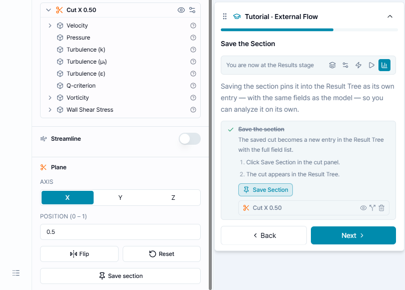
After saving, the cut appears in the Result Tree with the same field list as the original model. You can color the saved cut by Pressure, Velocity, or a turbulence field.
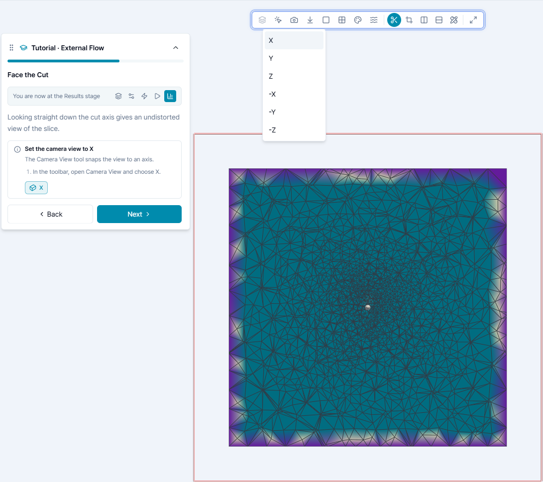
For a clean section view:
- Use the camera view tool and choose the same axis as the cut.
- Hide the main result body if it blocks the cut.
- Select the saved cut entry and choose a field such as Turbulence (k).
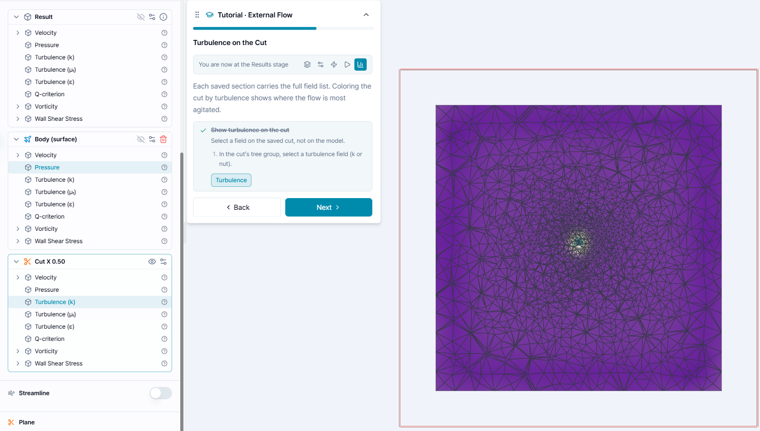
The saved section helps you inspect the flow core, mesh distribution, and turbulence concentration around the aircraft.
7. Results: Streamlines
Streamlines show how the flow moves through the domain.
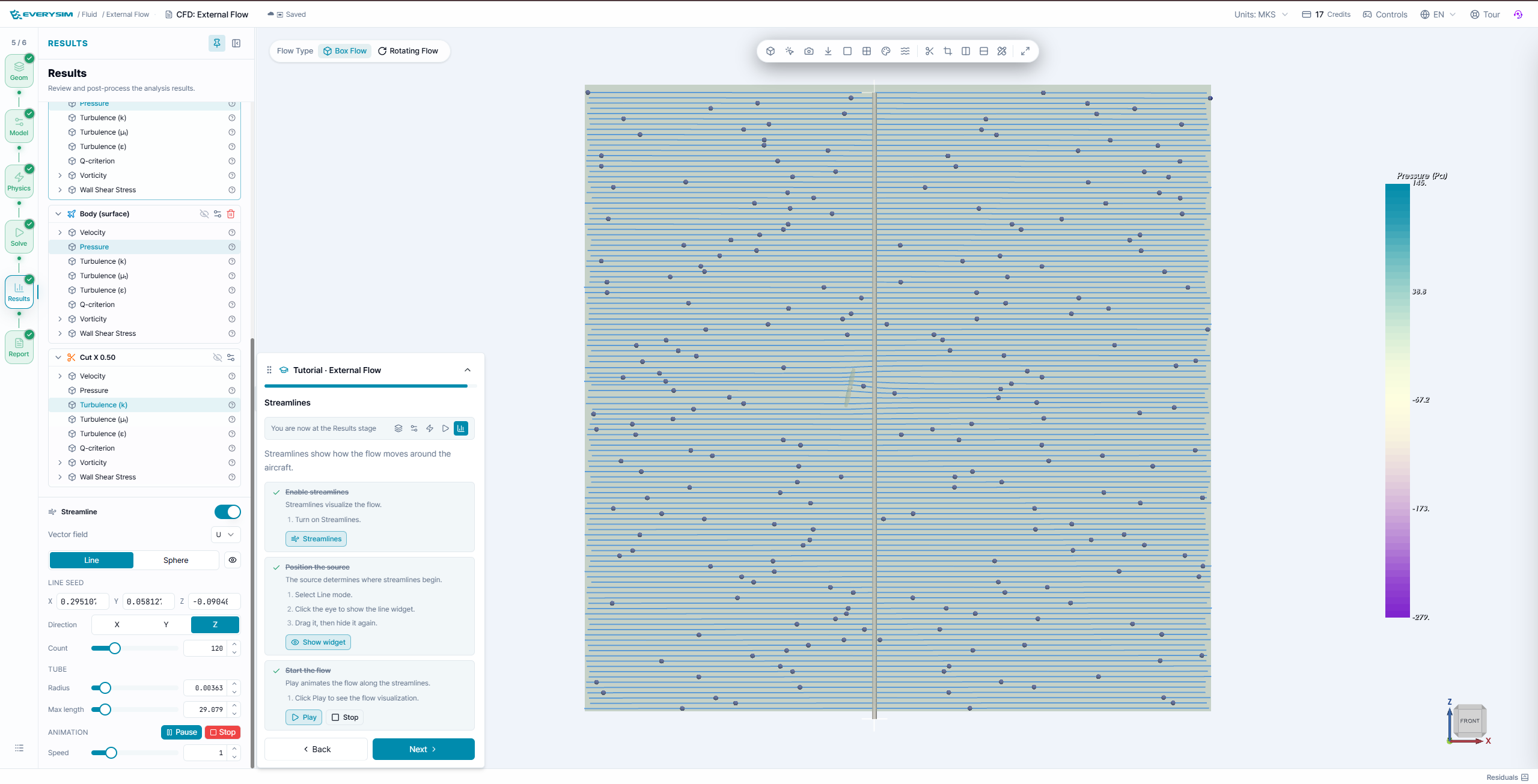
- Turn on Streamline.
- Select a vector field, such as velocity.
- Choose a line or sphere seed.
- Position the seed upstream of the aircraft.
- Adjust count, tube radius, maximum length, and speed as needed.
- Click Play to animate the flow.
Use streamlines to inspect whether air passes smoothly around the body, separates, or forms a disturbed wake.
8. Report
The Report stage turns the simulation into numerical summaries and charts.
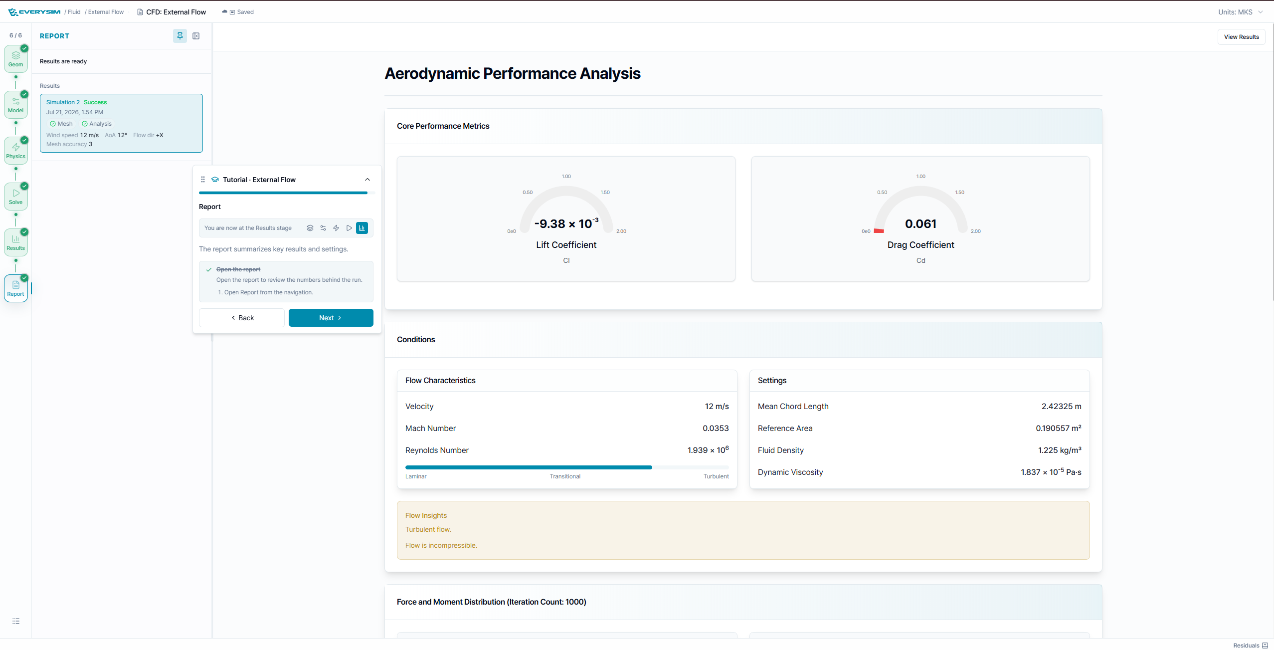
Start with the core performance metrics:
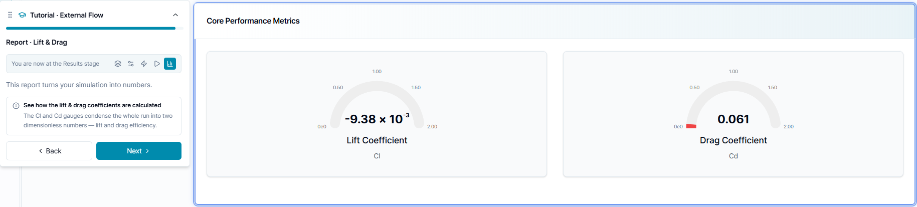
- Lift Coefficient (Cl): nondimensional lift value.
- Drag Coefficient (Cd): nondimensional drag value.
- Velocity, Mach Number, Reynolds Number: flow characteristics for interpreting the run.
- Reference Area, Mean Chord Length, Fluid Density, Dynamic Viscosity: settings used to calculate nondimensional quantities.
Then review force and moment distribution.
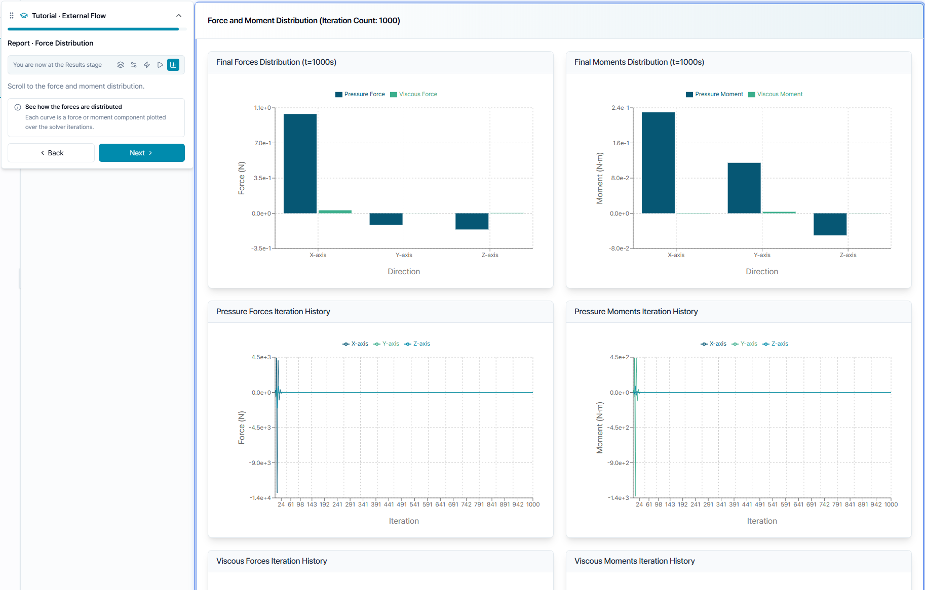
The bar charts show final pressure and viscous force/moment components by axis. The iteration histories show whether those values stabilize over time.
Practical Notes
- Use Box Flow for external aerodynamics around a body moving through air.
- Increase domain size if inlet, outlet, or side boundaries appear to influence the solution.
- Use higher accuracy when you need finer results, but expect longer solve times.
- Check residuals, field plots, cut planes, streamlines, and report trends together.
- If results look incorrect, review model scale, flow direction, angle of attack, lift direction, and whether the selected result field is displayed on the intended object.